Nico Addai

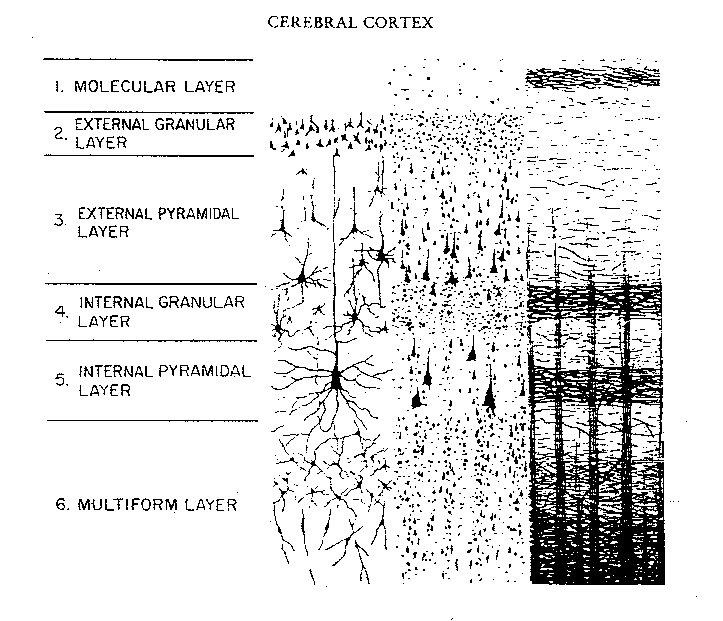
Using computation models, researchers are able to design network models which allow for the exploration in connectivity using both analysis and simulations. For the purposes of my Computational Neuroscience class, we’ll be focusing on neocortical circuits. The neocortex is the latest development in human evolution and is thought to be the location of higher processing, ie cognition. Let’s take it from the top!

What circuits in the brain are modeled using this?

Going forward, we’ll be dealing with the coordinate transformations needed in numerous situations including coordinate transformations needed in visually guided reach- ing, selective amplification leading to models of simple and complex cells in primary visual cortex, integration as a model of short-term memory, noise reduction, input selection, gain modulation, and associative memory. Networks must be unrelated with little synchronized firing where the precise patterns of spiking is unimportant.

Three Main Classes Modeled

1. Feedforward connections: This brings connections with input to a given region from another region located at an earlier stage along a particular processing pathway.
2. Top-down connections: Like in cognition, they connect signals from later stages in processing to earlier stages in processing.
3. Recurrent synapses: The most numerous connection in the circuit; it connects with other neurons at a similar level of processing.

One thing to note going forward: we won’t be replicating action potentials. Instead, we’ll be focusing on firing rates as APs are constrained by a time scale of milliseconds and take a lot of processing power. I’ve had my MATLab stall before when I used timescales of 0.1ms to model firing rates before! But why?

Arguments for Firing Rate Models

Also, using firing rates better replicates the stochasticity of neurons. Stochastic is an adjective that describes the quality of lacking any predictable order or plan. Neurons fire randomly, with irregular time intervals (Hence the use of rand and randi in MATLab to create random numbers).

It also also for more complicated reactions in a simplified network. Even though there are millions of cortical neurons receiving numerous inputs all the time, the probability of finding a synaptic connection between a randomly chosen pair of neurons is highly unlikely. By using firing rate models, we can average the probability of many networks at once in a way that we can’t with an all-or-nothing neuronal AP unit.

Arguments against Firing Rate Models

No model is perfect. One of the weaknesses of firing rates is in their strength: they are random. They cannot account for the spike timing- meaning that two spike have the potential to fire just half of the time an AP could fire. It also does not take into account spike correlations which is important for understanding the human nervous system.

Thanks for reading! This quarantine is helping me put pen to paper, and I will be posting a lot more, to VFA and beyond!